library(paneldesc)
library(tidyr)
library(gplots)
library(modelsummary)
library(plm)
library(fixest)
library(pdynmc)
library(xtsum)8 Comparison with other packages
Almost all of this package’s functionality can be replicated using individual functions from other packages. However, I believe the main advantage of the paneldesc package is that it combines all the functions necessary for panel data analysis and implements them in a single format. Below is a comparison with individual functions from other packages.
8.1 Set up
Import packages to compare.
8.2 Data import
Import the built-in dataset with simulated unbalanced panel data.
data(production)Create unbalanced panel for the analysis purposes.
unbalanced <- production[rowSums(!is.na(production[, c("sales", "capital", "labor", "industry")])) > 0, ]8.3 paneldesc vs. pdynmc
paneldesc::plot_patterns() and pdynmc::strucUPD.plot() visualize the participation patterns of entities in an unbalanced panel. pdynmc::strucUPD.plot() groups similar participation patterns by the number of periods and separates different patterns by bar color, while preserving the original order of the entities. In turn, paneldesc::plot_patterns() reorders entities by their patterns to show the dominance of each pattern using bar width.
paneldesc::plot_patterns(unbalanced, index = c("firm", "year"))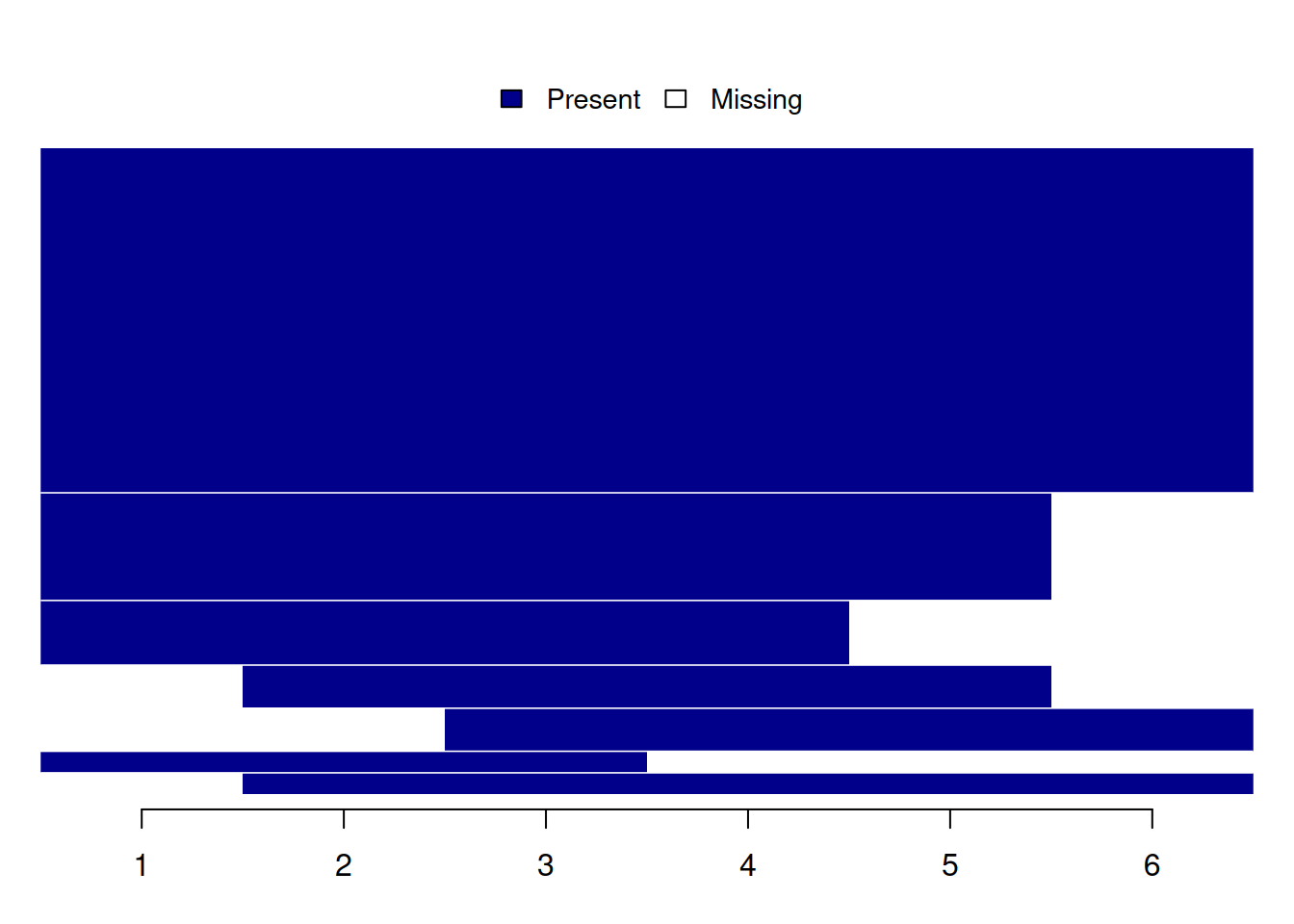
pdynmc::strucUPD.plot(unbalanced, i.name = "firm", t.name = "year")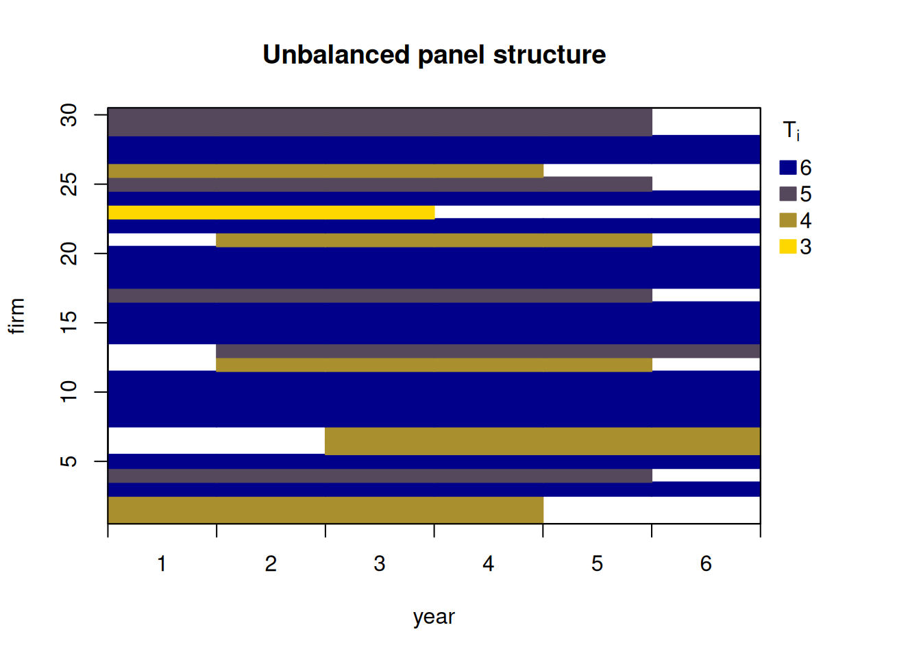
As can be seen above, the two functions produce similar results for an apparently unbalanced panel. However, applying pdynmc::strucUPD.plot() to the original production data frame results in an error, since it is technically balanced (the same number of years for each firm), while paneldesc::plot_patterns() detects entity-time pairs without other data and produces the same plot, showing the unbalanced panel structure.
paneldesc::plot_patterns(production, index = c("firm", "year"))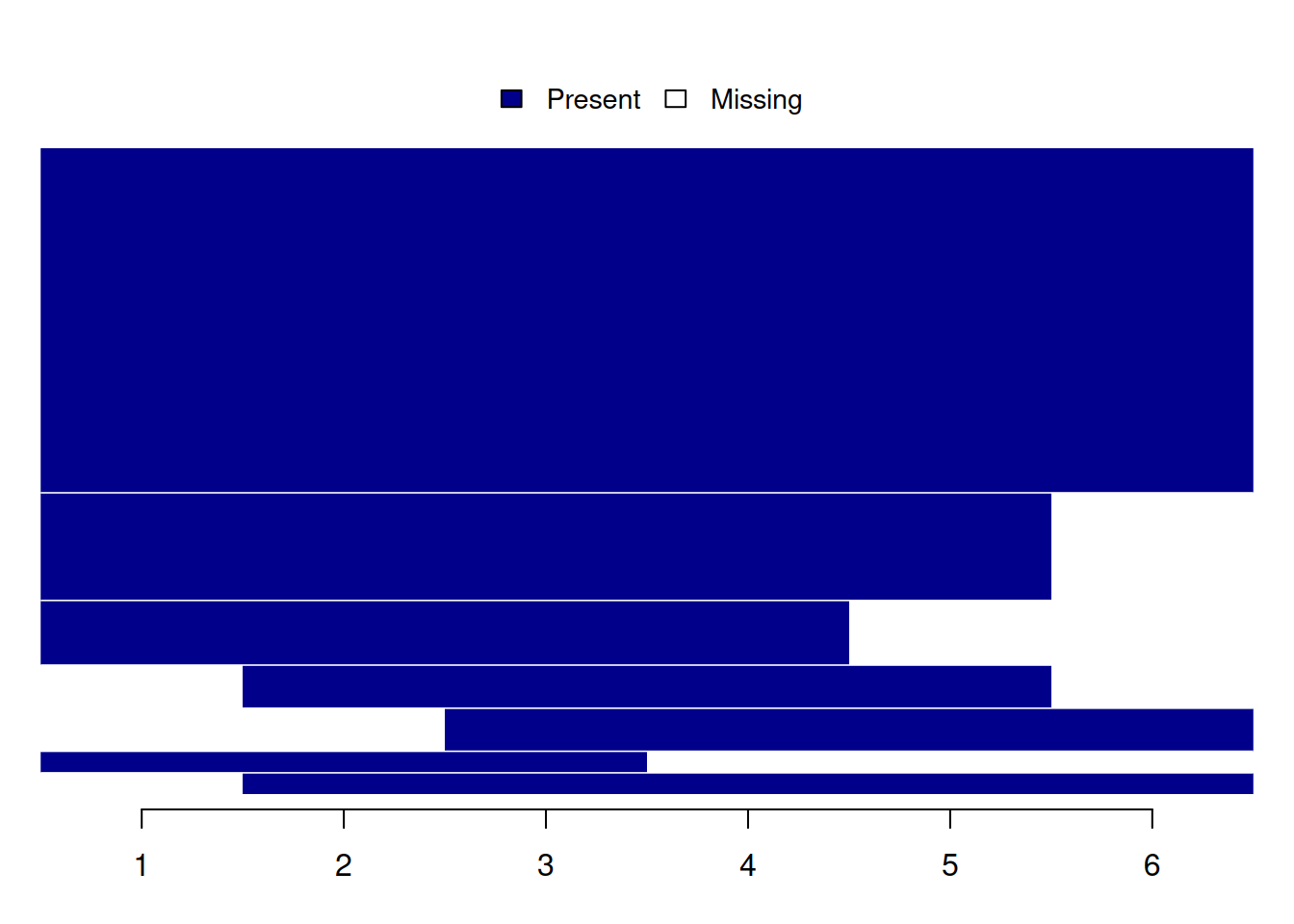
8.4 paneldesc vs. modelsummary
Among many other functions, paneldesc::summarize_numeric() and modelsummary::datasummary() provide tables with descriptive statistics for numeric variables and also allow the user to calculate statistics within groups. The main advantage of modelsummary::datasummary() is the flexibility of the output appearance, allowing various parameters to be specified for the table structure and output format. In turn, paneldesc::summarize_numeric() always returns a data frame, preserving the user’s freedom of further work with it. Furthermore, in my opinion, the syntax of paneldesc::summarize_numeric() is simpler compared to modelsummary::datasummary(), although this is a matter of taste.
paneldesc::summarize_numeric(
  production,
  select = c("capital", "labor"),
  group = "year"
)| year | variable | count | mean | std | min | max |
|---|---|---|---|---|---|---|
| 1 | capital | 25 | 40.154 | 39.004 | 3.206 | 148.942 |
| 1 | labor | 24 | 74.349 | 69.766 | 18.414 | 333.377 |
| 2 | capital | 28 | 30.210 | 30.596 | 5.032 | 122.332 |
| 2 | labor | 28 | 81.758 | 66.571 | 17.666 | 327.581 |
| 3 | capital | 28 | 30.111 | 30.372 | 2.030 | 121.740 |
| 3 | labor | 29 | 82.256 | 106.869 | 8.172 | 579.024 |
| 4 | capital | 28 | 34.889 | 32.046 | 7.146 | 148.994 |
| 4 | labor | 29 | 55.533 | 46.448 | 5.972 | 207.572 |
| 5 | capital | 26 | 28.076 | 21.871 | 4.637 | 78.244 |
| 5 | labor | 25 | 74.056 | 71.255 | 15.879 | 266.829 |
| 6 | capital | 19 | 37.145 | 39.400 | 3.690 | 160.085 |
| 6 | labor | 19 | 101.003 | 67.261 | 18.669 | 259.851 |
modelsummary::datasummary(
  Factor(year) * (capital + labor) ~ N + Mean + SD + Min + Max,
  data = production
)| year | N | Mean | SD | Min | Max | |
|---|---|---|---|---|---|---|
| 1 | capital | 25 | 40.15 | 39.00 | 3.21 | 148.94 |
| labor | 24 | 74.35 | 69.77 | 18.41 | 333.38 | |
| 2 | capital | 28 | 30.21 | 30.60 | 5.03 | 122.33 |
| labor | 28 | 81.76 | 66.57 | 17.67 | 327.58 | |
| 3 | capital | 28 | 30.11 | 30.37 | 2.03 | 121.74 |
| labor | 29 | 82.26 | 106.87 | 8.17 | 579.02 | |
| 4 | capital | 28 | 34.89 | 32.05 | 7.15 | 148.99 |
| labor | 29 | 55.53 | 46.45 | 5.97 | 207.57 | |
| 5 | capital | 26 | 28.08 | 21.87 | 4.64 | 78.24 |
| labor | 25 | 74.06 | 71.26 | 15.88 | 266.83 | |
| 6 | capital | 19 | 37.15 | 39.40 | 3.69 | 160.08 |
| labor | 19 | 101.00 | 67.26 | 18.67 | 259.85 |
8.5 paneldesc vs. gplots
The functions paneldesc::plot_heterogeneity() and gplots::plotmeans() allow the user to analyze heterogeneity between and within groups. The results of these functions are quite similar: they visualize group means and the within-group variance of the selected variable. The main difference is that gplots::plotmeans() displays group size labels and plots confidence intervals, while paneldesc::plot_heterogeneity() plots a point for each observation to show both the variance and the group size.
paneldesc::plot_heterogeneity(production, select = "sales", group = "year")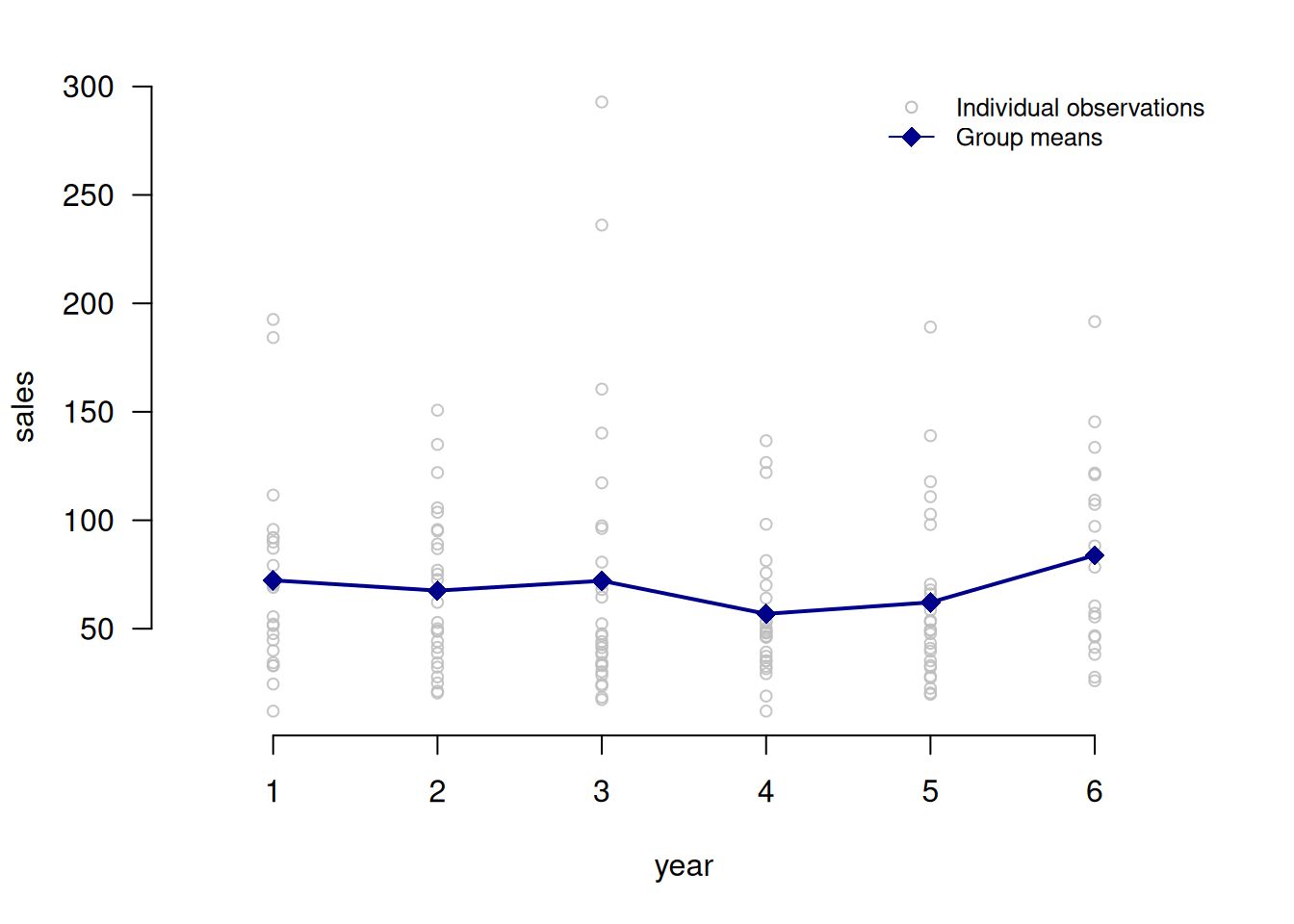
gplots::plotmeans(sales ~ year, production)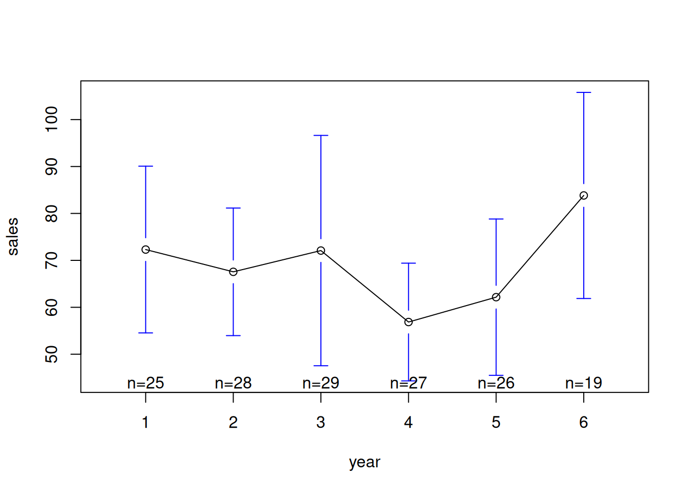
8.6 paneldesc vs. xtsum
paneldesc::decompose_numeric() and xtsum::xtsum() provide descriptive statistics for numeric variables in panel data. Specifically, they decompose the standard deviation into between-value and within-value components, mimicking the xtsum command in Stata. The syntax and behavior of the functions are quite similar. By default, xtsum::xtsum() returns output in HTML format, although it allows customization. In turn, paneldesc::summarize_numeric() always returns a data frame, preserving the user’s freedom for further manipulation.
paneldesc::decompose_numeric(
  production,
  select = c("sales", "capital", "labor"),
  index = "firm"
)| variable | dimension | mean | std | min | max | count |
|---|---|---|---|---|---|---|
| sales | overall | 68.402 | 45.025 | 11.999 | 292.850 | 154.000 |
| sales | between | NA | 29.060 | 34.263 | 166.364 | 30.000 |
| sales | within | NA | 34.127 | -12.444 | 234.297 | 5.133 |
| capital | overall | 33.152 | 32.044 | 2.030 | 160.085 | 154.000 |
| capital | between | NA | 17.414 | 9.019 | 74.225 | 30.000 |
| capital | within | NA | 27.072 | -25.567 | 149.329 | 5.133 |
| labor | overall | 76.883 | 74.150 | 5.972 | 579.024 | 154.000 |
| labor | between | NA | 41.068 | 31.021 | 190.645 | 30.000 |
| labor | within | NA | 61.202 | -58.040 | 483.217 | 5.133 |
xtsum::xtsum(
  production,
  variables = c("sales", "capital", "labor"),
  id = "firm",
  t = "year",
  na.rm = TRUE
)| Variable | Dim | Mean | SD | Min | Max | Observations |
|---|---|---|---|---|---|---|
| ___________ | _________ | |||||
| sales | overall | 68.402 | 45.025 | 11.999 | 292.85 | N = 154 |
| between | 29.06 | 34.263 | 166.364 | n = 30 | ||
| within | 34.127 | -12.444 | 234.297 | T = 5.133 | ||
| ___________ | _________ | |||||
| capital | overall | 33.152 | 32.044 | 2.03 | 160.085 | N = 154 |
| between | 17.414 | 9.019 | 74.225 | n = 30 | ||
| within | 27.072 | -25.567 | 149.329 | T = 5.133 | ||
| ___________ | _________ | |||||
| labor | overall | 76.883 | 74.15 | 5.972 | 579.024 | N = 154 |
| between | 41.068 | 31.021 | 190.645 | n = 30 | ||
| within | 61.202 | -58.04 | 483.217 | T = 5.133 |
8.7 paneldesc vs. plm
paneldesc::make_balanced() and plm::make.pbalanced() allow the user to obtain various types of balanced panel datasets.
paneldesc_bal_1 <- paneldesc::make_balanced(
  unbalanced,
  index = c("firm", "year"),
  balance = "entities"
)
dim(paneldesc_bal_1)
[1] 96 8paneldesc_bal_2 <- paneldesc::make_balanced(
unbalanced,
index = c("firm", "year"),
balance = "periods"
)
dim(paneldesc_bal_2)[1] 30 8paneldesc_bal_3 <- paneldesc::make_balanced(
unbalanced,
index = c("firm", "year"),
balance = "rows"
)
dim(paneldesc_bal_3)[1] 180 8plm_bal_1 <- plm::make.pbalanced(
unbalanced,
index = c("firm", "year"),
balance.type = "shared.individuals"
)
dim(plm_bal_1)[1] 96 8plm_bal_2 <- plm::make.pbalanced(
unbalanced,
index = c("firm", "year"),
balance.type = "shared.times"
)
dim(plm_bal_2)[1] 30 8plm_bal_3 <- plm::make.pbalanced(
unbalanced,
index = c("firm", "year"),
balance.type = "fill"
)
dim(plm_bal_3)[1] 180 8As can be seen above, the two functions produce similar results for an apparently unbalanced panel. However, applying plm::make.pbalanced() to the original production dataframe results in no changes, as it is technically balanced (the same number of years for each firm), while paneldesc::make_balanced() automatically detects entity-time pairs without other data, revealing the unbalanced panel structure. This allows the function to balance the panel in the same way as shown above.
paneldesc_bal_1b <- paneldesc::make_balanced(
  production,
  index = c("firm", "year"),
  balance = "entities"
)
dim(paneldesc_bal_1b)
[1] 96 8paneldesc_bal_2b <- paneldesc::make_balanced(
production,
index = c("firm", "year"),
balance = "periods"
)
dim(paneldesc_bal_2b)[1] 30 8paneldesc_bal_3b <- paneldesc::make_balanced(
production,
index = c("firm", "year"),
balance = "rows"
)
dim(paneldesc_bal_3b)[1] 180 8plm_bal_1b <- plm::make.pbalanced(
production,
index = c("firm", "year"),
balance.type = "shared.individuals"
)
dim(plm_bal_1b)[1] 180 8plm_bal_2b <- plm::make.pbalanced(
production,
index = c("firm", "year"),
balance.type = "shared.times"
)
dim(plm_bal_2b)[1] 180 8plm_bal_3b <- plm::make.pbalanced(
production,
index = c("firm", "year"),
balance.type = "fill"
)
dim(plm_bal_3b)[1] 180 88.8 paneldesc vs. fixest
paneldesc::make_demeaned() and fixest::demean() allow the user to demean variables using various grouping patterns. As can be seen below, basic applications of these functions to a single variable produce similar results. When working with multiple variables, the behavior of the functions differs slightly. fixest::demean() is aimed at regression analysis and therefore removes all rows with missing values for at least one variable and performs calculations based on the resulting dataset. paneldesc::make_demeaned(), in contrast, preserves missing values in the dataset and performs transformations on the full dataset (when calculating within-group means, missing values are removed for each variable separately, which often allows for more data to be used compared to fixest::demean()). Thus, the paneldesc::make_demeaned() function may be preferable for exploratory data analysis, as it preserves more observations. In turn, fixest::demean() is more flexible in configuration, allowing the user to select many additional parameters.
demeaned_paneldesc <- paneldesc::make_demeaned(
    production[, c("sales", "firm", "year")],
    group = c("firm", "year")
)
Demeaning numeric variables: salessummary(demeaned_paneldesc) sales firm year
Min. :-75.9166 Min. : 1.0 Min. :1.0
1st Qu.:-22.7824 1st Qu.: 8.0 1st Qu.:2.0
Median : -0.6208 Median :15.5 Median :3.5
Mean : 0.0000 Mean :15.5 Mean :3.5
3rd Qu.: 16.3642 3rd Qu.:23.0 3rd Qu.:5.0
Max. :163.1807 Max. :30.0 Max. :6.0
NA's :26 demeaned_fixest <- fixest::demean(
X = production[, "sales"],
f = production[, c("firm", "year")]
)NOTE: 26 observations removed because of NA values (Breakup: X: 26, f: 0).summary(demeaned_fixest) V1
Min. :-75.9166
1st Qu.:-22.7824
Median : -0.6208
Mean : 0.0000
3rd Qu.: 16.3642
Max. :163.1807 8.9 paneldesc vs. tidyr
Among other functions, paneldesc::make_wide() and paneldesc::make_long(), as well as tidyr::pivot_wider() and tidyr::pivot_longer(), allow the user to transform panel data from long to wide format and from wide to long, respectively. The key advantage of the paneldesc functions is their simpler and more automatic implementation in a panel data context, including the ability to handle time-varying and static variables separately. In turn, the tidyr functions are more adaptable for a broader range of applications, although they lack automatic solutions for panel data. For example, the region variable in the production dataset is a time-invariant variable, but has missing observations due to the unbalanced structure of the panel data. In this case, the tidyr functions require data preprocessing, which somewhat complicates their implementation (omitted here for brevity). Also, I find the syntax of the paneldesc function simpler than tidyr, although that’s a matter of taste.
wide_paneldesc <- paneldesc::make_wide(
    production,
    select = c("sales", "capital", "labor", "industry", "ownership"),
    index = c("firm", "year")
)
Static variables: region
Reshaped variables: sales_1, sales_2, sales_3, sales_4, sales_5, sales_6
capital_1, capital_2, capital_3, capital_4, capital_5, capital_6
labor_1, labor_2, labor_3, labor_4, labor_5, labor_6
industry_1, industry_2, industry_3, industry_4, industry_5, industry_6
ownership_1, ownership_2, ownership_3, ownership_4, ownership_5, ownership_6 long_paneldesc <- paneldesc::make_long(
wide_paneldesc,
select = c("sales", "capital", "labor", "industry", "ownership"),
index = c("firm", "year")
) Static variables: region
Reshaped variables: sales, capital, labor, industry, ownership wide_tidyr <- tidyr::pivot_wider(
production,
id_cols = firm,
names_from = year,
values_from = !c(firm, year)
)
names(wide_tidyr) [1] "firm" "sales_1" "sales_2" "sales_3" "sales_4"
[6] "sales_5" "sales_6" "capital_1" "capital_2" "capital_3"
[11] "capital_4" "capital_5" "capital_6" "labor_1" "labor_2"
[16] "labor_3" "labor_4" "labor_5" "labor_6" "industry_1"
[21] "industry_2" "industry_3" "industry_4" "industry_5" "industry_6"
[26] "ownership_1" "ownership_2" "ownership_3" "ownership_4" "ownership_5"
[31] "ownership_6" "region_1" "region_2" "region_3" "region_4"
[36] "region_5" "region_6" long_tidyr <- tidyr::pivot_longer(
wide_tidyr,
cols = !firm,
names_to = c(".value", "year"),
names_pattern = "(.*)_(.*)"
)
names(long_tidyr)[1] "firm" "year" "sales" "capital" "labor" "industry"
[7] "ownership" "region"