5 Extended example – paneldesc package guides

5.1 Set up

Import the package.

library(paneldesc)

5.2 Data import

Import the built-in dataset with simulated unbalanced panel data.

data(production)

Set up a panel structure in advance so that you don’t have to do it later each time you use other functions. Note that if delta is supplied, the function checks for omitted time periods. If such periods exist, they will be taken into account when other functions work with this argument.

panel <- make_panel(production, index = c("firm", "year"), delta = 1)

5.3 Creating balanced panel data

The make_panel() function also allows to balance panel data using various options:

keeping only entities present in all time periods;

balance_entities <- make_panel(production, index = c("firm", "year"), balance = "entities")

keeping only time periods where all entities are present;

balance_periods <- make_panel(production, index = c("firm", "year"), balance = "periods")

creating a row for every entity‑time combination (if delta is supplied, the full time sequence including missing periods is used).

balance_rows <- make_panel(production, index = c("firm", "year"), delta = 1, balance = "rows")

5.4 Panel data structure analysis

If necessary, you can display more detailed statistics on the distribution of entities by periods and periods by entities.

describe_balance(panel, detail = TRUE, digits = 2)

dimension	mean	std	min	p5	p25	p50	p75	p95	max
entities	26.17	3.97	19	20.5	25.25	27	28.75	29.75	30
periods	5.23	0.94	3	4.0	4.25	6	6.00	6.00	6

plot_periods() function allows to customize colors.

plot_periods(panel, colors = c("gray", "black"))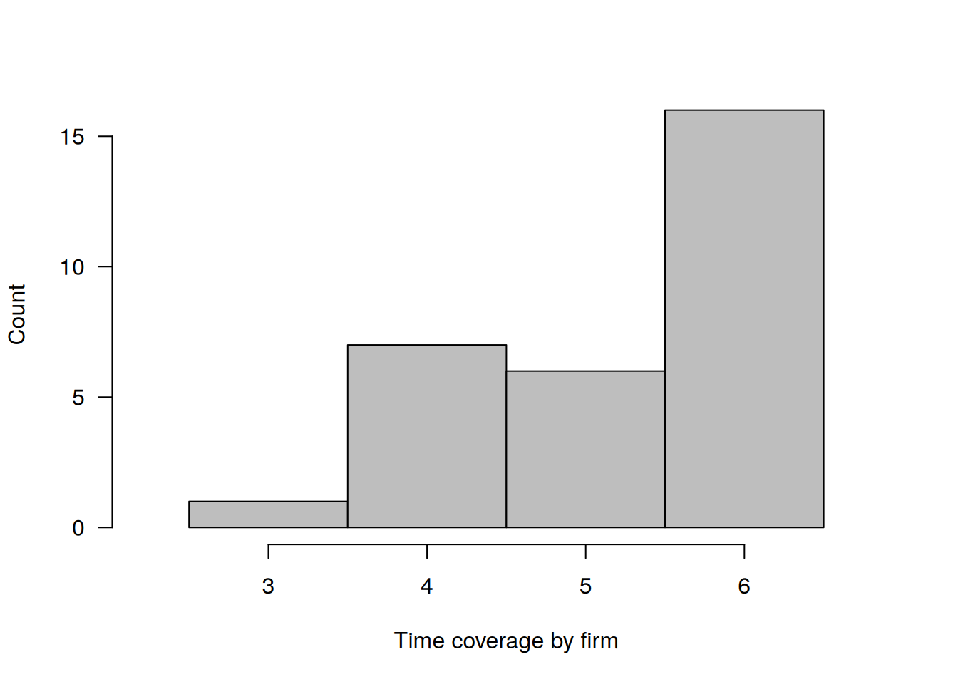

Both describe_patterns() and plot_patterns() allow you to limit the range of patterns to display. In addition, desribe_patterns() allows to customize rounding when calculting shares, while plot_patterns() allows to customize colors.

describe_patterns(panel, limits = 3, digits = 2)

pattern	1	2	3	4	5	6	count	share
1	1	1	1	1	1	1	16	0.53
2	1	1	1	1	1	0	5	0.17
3	1	1	1	1	0	0	3	0.10

plot_patterns(panel, limits = c(4, 6), colors = c("darkgray", "white"))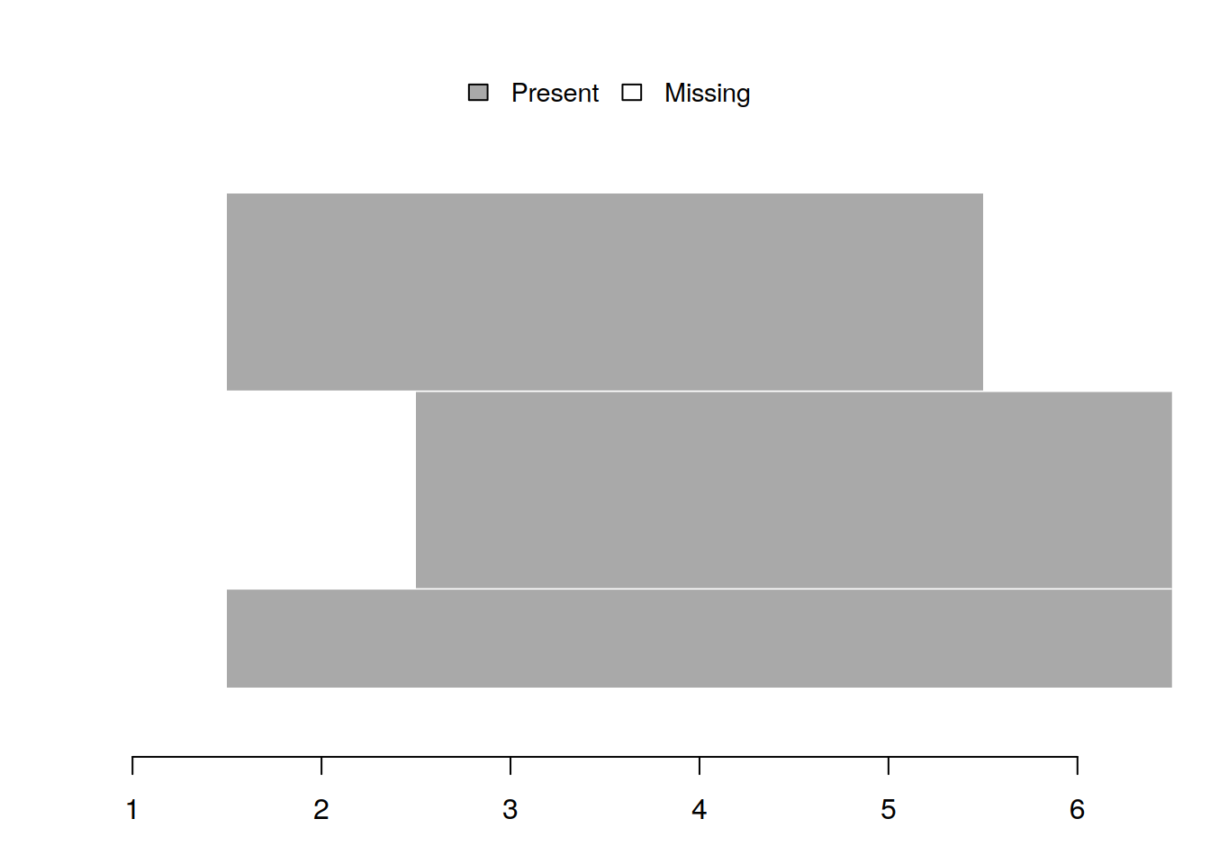

5.5 Missing values analysis

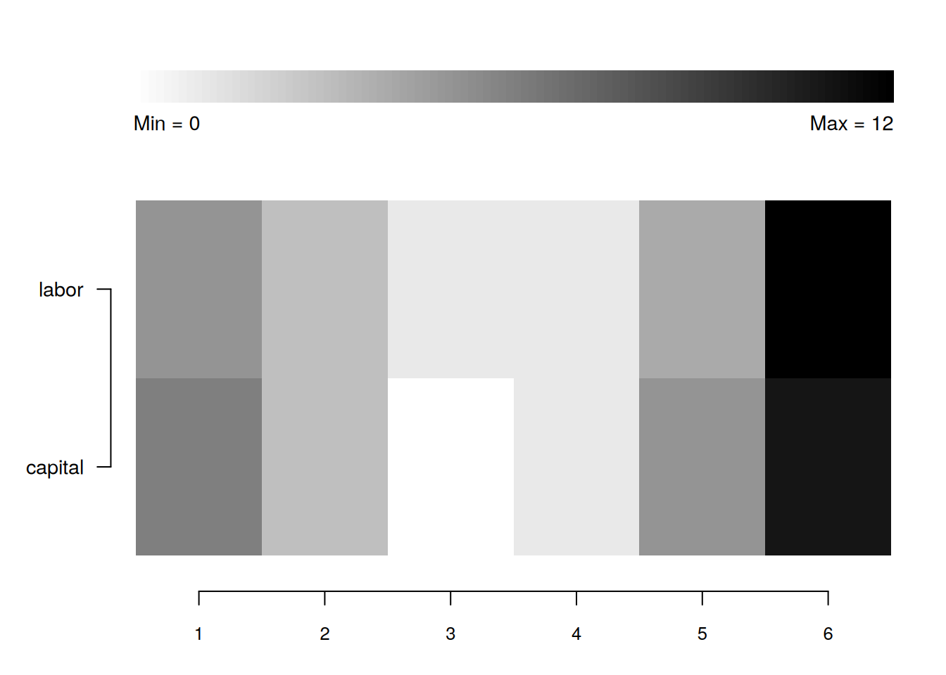
plot_missing() allows to select specific variables to analyze. One can also customize colors.

plot_missing(
  panel,
  select = c("labor", "capital"),
  colors = c("black", "white")
)

summarize_missing() also allows to select specific variables to analyze. In addition, it can provide more detailed table by adding period-specific missing value counts. One can also customize rounding.

summarize_missing(
  panel,
  select = c("labor", "capital"),
  detail = TRUE,
  digits = 2
)

variable	na_count	na_share	entities	periods	1	2	3	4	5	6
labor	26	0.14	16	6	5	3	1	1	4	12
capital	26	0.14	17	5	6	3	0	1	5	11

describe_incomplete() can provide more detailed table by adding variable-specific missing value counts.

describe_incomplete(panel, detail = TRUE)

firm	na_count	variables	sales	capital	labor	industry	ownership
23	15	5	3	3	3	3	3
21	11	5	3	2	2	2	2
1	10	5	2	2	2	2	2
2	10	5	2	2	2	2	2
6	10	5	2	2	2	2	2
7	10	5	2	2	2	2	2
12	10	5	2	2	2	2	2
26	10	5	2	2	2	2	2
25	6	5	1	1	2	1	1
30	6	5	2	1	1	1	1
4	5	5	1	1	1	1	1
13	5	5	1	1	1	1	1
17	5	5	1	1	1	1	1
29	5	5	1	1	1	1	1
8	2	2	0	1	1	0	0
3	1	1	0	0	1	0	0
10	1	1	0	1	0	0	0
14	1	1	1	0	0	0	0
24	1	1	0	1	0	0	0

5.6 Numeric variables analysis

summarize_numeric() allows to select specific variables to analyze. It also can provide additional statisitcs. Custom rounding is also available.

summarize_numeric(
  panel,
  select = c("sales", "labor"),
  group = "year",
  detail = TRUE,
  digits = 2
)

year	variable	count	mean	std	min	p25	p50	p75	max
1	sales	25	58.49	44.59	8.32	26.36	44.74	74.58	190.10
1	labor	25	68.87	66.94	4.10	20.88	39.44	96.76	246.85
2	sales	28	56.10	37.94	17.80	31.87	40.78	73.49	186.35
2	labor	27	60.46	48.48	11.69	30.04	45.41	69.00	222.76
3	sales	30	76.66	47.57	20.58	42.90	70.74	96.91	219.51
3	labor	29	90.44	82.63	9.28	40.92	62.88	114.85	414.84
4	sales	28	73.10	33.24	19.46	46.96	72.90	99.39	135.12
4	labor	29	73.97	54.00	16.33	34.23	58.99	96.46	240.73
5	sales	24	75.40	43.09	20.16	43.47	70.76	95.08	211.09
5	labor	26	90.60	85.03	21.06	35.90	73.02	99.07	413.78
6	sales	19	81.74	73.32	20.35	41.90	67.33	85.09	336.85
6	labor	18	96.61	103.78	20.51	37.10	55.89	111.35	419.85

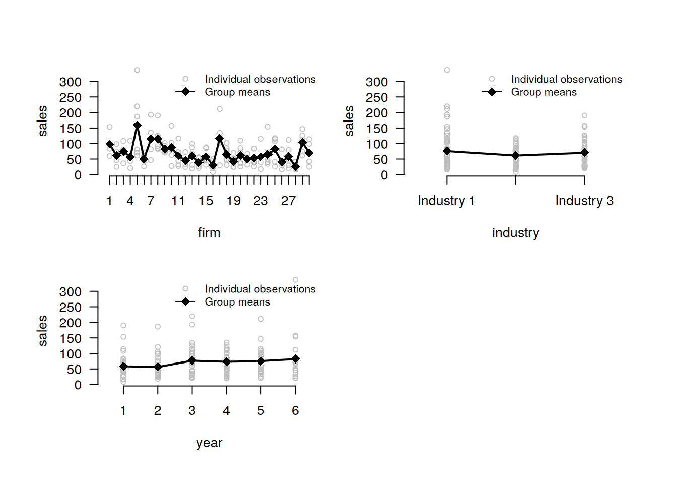
plot_heterogeneity() allows to choose several grouping variables. One can also customize colors.

plot_heterogeneity(
  panel,
  select = "sales",
  group = c("firm", "industry", "year"),
  colors = c("black", "gray")
)

decompose_numeric() allows to select specific varibles to analyze. One also can output the resulting table in wide format and hide redundant details, as well as customize rounding.

decompose_numeric(
  panel,
  select = c("sales", "labor"),
  detail = FALSE,
  format = "wide",
  digits = 2
)

variable	mean	std_overall	std_between	std_within
sales	69.76	46.80	29.78	35.86
labor	79.33	73.69	44.02	59.56

5.7 Factor variables analysis

Compared to the default settings, both decompose_factor() and summarize_transition() functions can output the resulting table in long format and also allow to customize rounding. descompose_factor() also allows to select specific variables to analyze.

decompose_factor(panel, select = "industry", format = "long", digits = 2)

variable	category	dimension	count	share
industry	Industry 1	between	13	0.43
industry	Industry 2	between	11	0.37
industry	Industry 3	between	10	0.33
industry	Industry 1	overall	63	0.40
industry	Industry 2	overall	45	0.29
industry	Industry 3	overall	49	0.31
industry	Industry 1	within	NA	0.92
industry	Industry 2	within	NA	0.81
industry	Industry 3	within	NA	0.92

summarize_transition(panel, select = "industry", format = "long", digits = 2)

23 rows with NA values in 'industry' removed.

from	to	count	share
Industry 1	Industry 1	50	1.00
Industry 1	Industry 2	0	0.00
Industry 1	Industry 3	0	0.00
Industry 2	Industry 1	2	0.05
Industry 2	Industry 2	34	0.92
Industry 2	Industry 3	1	0.03
Industry 3	Industry 1	0	0.00
Industry 3	Industry 2	1	0.03
Industry 3	Industry 3	39	0.98