7  Comparison with other packages

Almost all of this package’s functionality can be replicated using individual functions from other packages. However, I believe the main advantage of the paneldesc package is that it combines all the functions necessary for panel data analysis and implements them in a single format. Below is a comparison with individual functions from other packages.

7.1 Set up

Import packages to compare.

library(paneldesc)
library(gplots)
library(modelsummary)
library(plm)
library(pdynmc)
library(xtsum)

7.2 Data import

Import the built-in dataset with simulated unbalanced panel data.

data(production)

Create unbalanced panel for the analysis purposes.

unbalanced <- production[rowSums(!is.na(production[, c("sales", "capital", "labor", "industry")])) > 0, ]

7.3 paneldesc vs. pdynmc

paneldesc::plot_patterns(production, index = c("firm", "year"))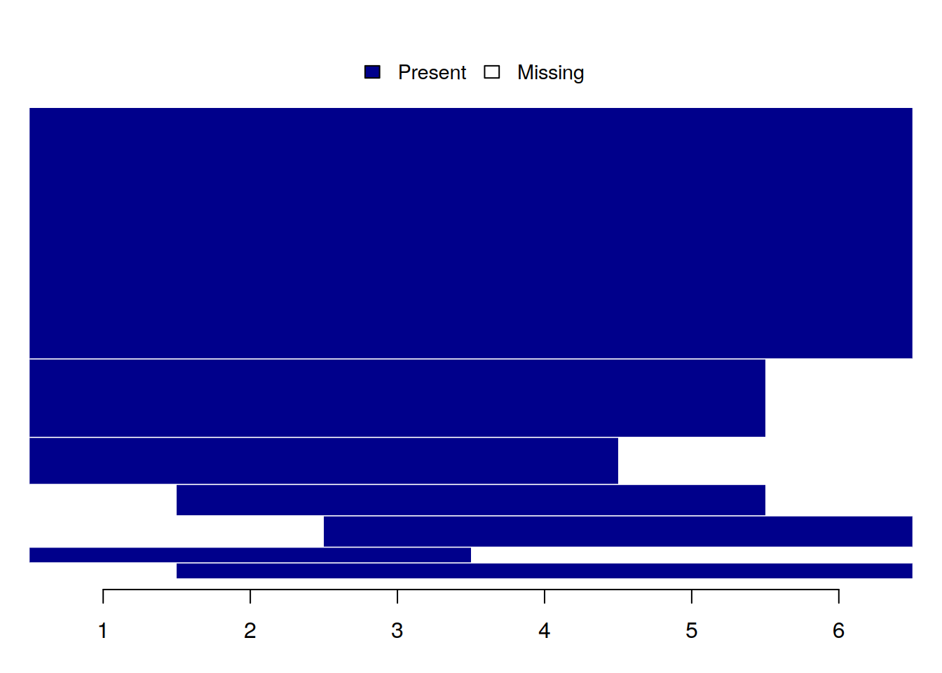

pdynmc::strucUPD.plot(unbalanced, i.name = "firm", t.name = "year")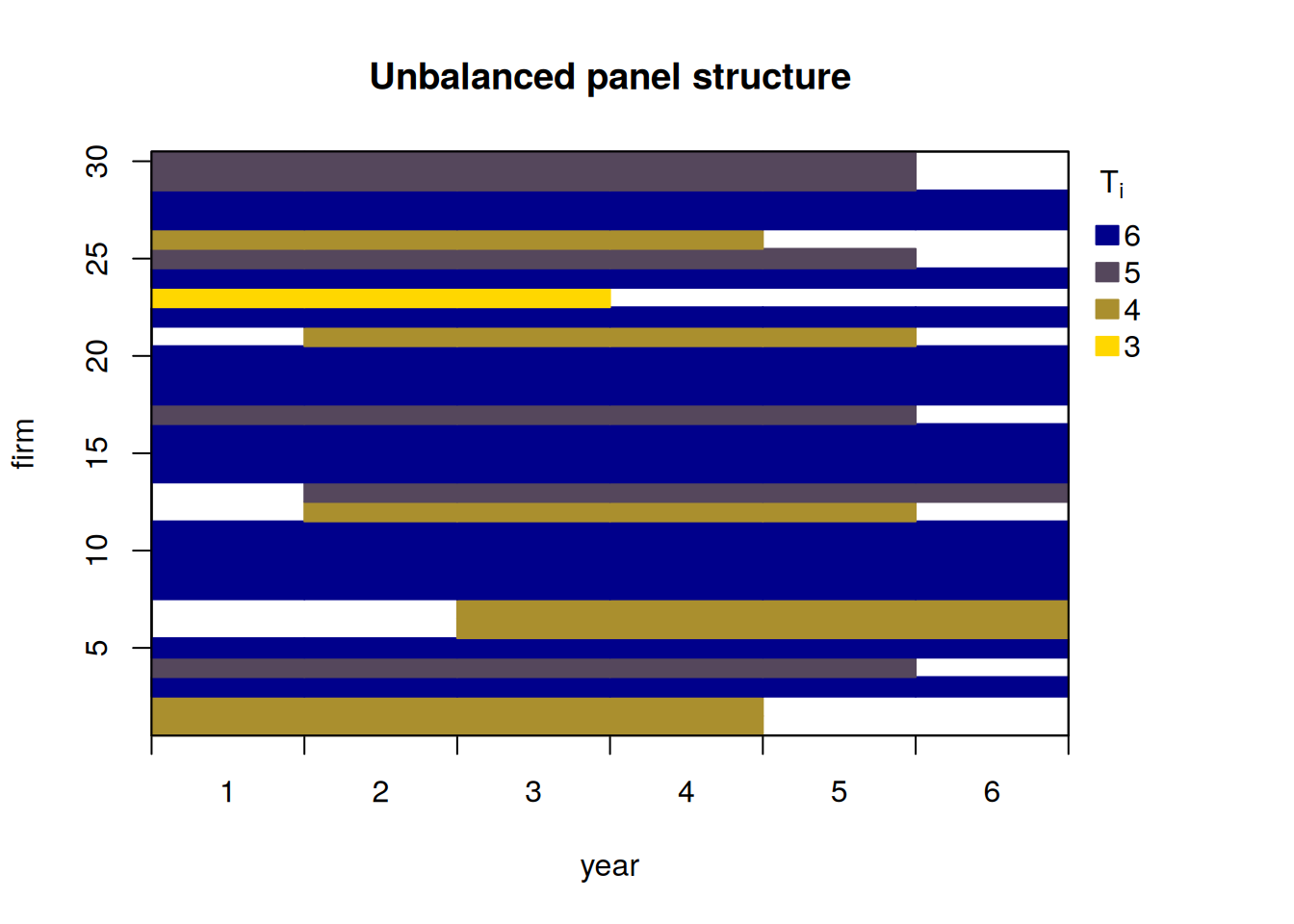

7.4 paneldesc vs. modelsummary

paneldesc::summarize_numeric(production, select = c("capital", "labor"), group = "year")

year	variable	count	mean	std	min	max
1	capital	24	24.862	16.273	0.968	65.950
1	labor	25	68.871	66.941	4.097	246.852
2	capital	27	28.790	31.053	3.150	151.464
2	labor	27	60.463	48.484	11.692	222.761
3	capital	30	35.464	39.174	4.729	194.719
3	labor	29	90.437	82.628	9.284	414.844
4	capital	29	44.522	35.375	5.080	132.898
4	labor	29	73.967	54.005	16.327	240.726
5	capital	25	28.351	23.127	5.339	86.078
5	labor	26	90.604	85.026	21.063	413.784
6	capital	19	29.767	30.908	2.288	108.787
6	labor	18	96.609	103.777	20.507	419.848

modelsummary::datasummary(Factor(year) * (capital + labor) ~ N + Mean + SD + Min + Max, data = production)

year		N	Mean	SD	Min	Max
1	capital	24	24.86	16.27	0.97	65.95
	labor	25	68.87	66.94	4.10	246.85
2	capital	27	28.79	31.05	3.15	151.46
	labor	27	60.46	48.48	11.69	222.76
3	capital	30	35.46	39.17	4.73	194.72
	labor	29	90.44	82.63	9.28	414.84
4	capital	29	44.52	35.38	5.08	132.90
	labor	29	73.97	54.00	16.33	240.73
5	capital	25	28.35	23.13	5.34	86.08
	labor	26	90.60	85.03	21.06	413.78
6	capital	19	29.77	30.91	2.29	108.79
	labor	18	96.61	103.78	20.51	419.85

7.5 paneldesc vs. gplots

paneldesc::plot_heterogeneity(production, select = "sales", group = "year")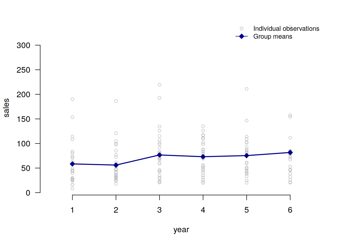

gplots::plotmeans(sales ~ year, production)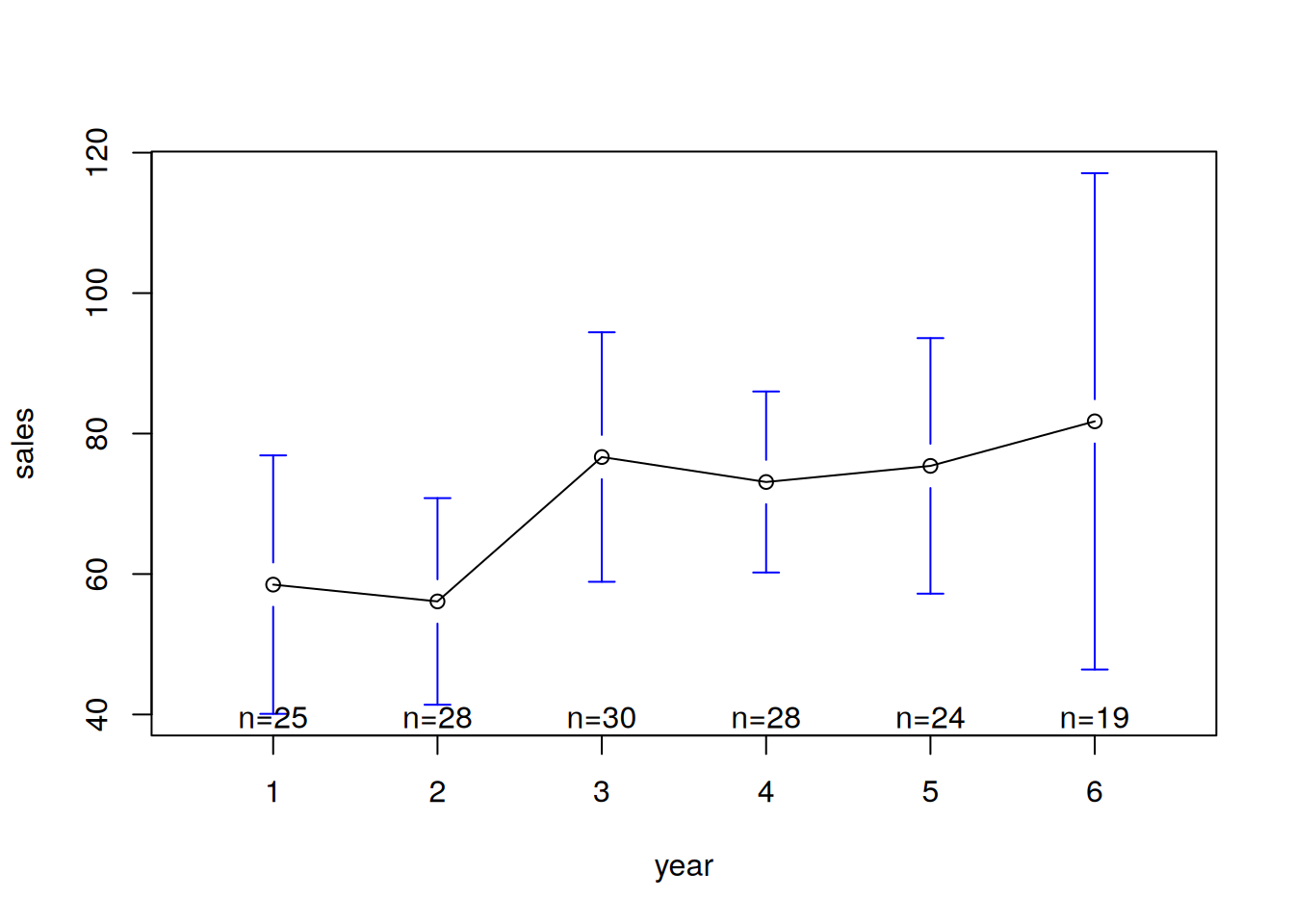

7.6 paneldesc vs. xtsum

paneldesc::decompose_numeric(production, select = c("sales", "capital", "labor"), index = "firm")

variable	dimension	mean	std	min	max	count
sales	overall	69.756	46.804	8.321	336.853	154.000
sales	between	NA	29.776	25.772	159.197	30.000
sales	within	NA	35.862	-28.397	247.412	5.133
capital	overall	32.490	31.053	0.968	194.719	154.000
capital	between	NA	13.969	8.671	75.083	30.000
capital	within	NA	27.701	-22.444	152.126	5.133
labor	overall	79.329	73.687	4.097	419.848	154.000
labor	between	NA	44.023	24.606	175.731	30.000
labor	within	NA	59.561	-77.709	323.445	5.133

xtsum::xtsum(production, variables = c("sales", "capital", "labor"), id = "firm", t = "year", na.rm = TRUE)

Variable	Dim	Mean	SD	Min	Max	Observations
___________	_________
sales	overall	69.756	46.804	8.321	336.853	N = 154
	between		29.776	25.772	159.197	n = 30
	within		35.862	-28.397	247.412	T = 5.133
___________	_________
capital	overall	32.49	31.053	0.968	194.719	N = 154
	between		13.969	8.671	75.083	n = 30
	within		27.701	-22.444	152.126	T = 5.133
___________	_________
labor	overall	79.329	73.687	4.097	419.848	N = 154
	between		44.023	24.606	175.731	n = 30
	within		59.561	-77.709	323.445	T = 5.133

7.7 paneldesc vs. plm

paneldesc_bal_1 <- paneldesc::make_panel(unbalanced, index = c("firm", "year"), balance = "entities")
dim(paneldesc_bal_1)

[1] 96  7

paneldesc_bal_2 <- paneldesc::make_panel(unbalanced, index = c("firm", "year"), balance = "periods")
dim(paneldesc_bal_2)

[1] 30  7

paneldesc_bal_3 <- paneldesc::make_panel(unbalanced, index = c("firm", "year"), balance = "rows")
dim(paneldesc_bal_3)

[1] 180   7

unbalanced_pdata <- plm::pdata.frame(unbalanced, index = c("firm", "year"))

plm_bal_1 <- plm::make.pbalanced(unbalanced_pdata, balance.type = "shared.individuals")
dim(plm_bal_1)

[1] 96  7

plm_bal_2 <- plm::make.pbalanced(unbalanced_pdata, balance.type = "shared.times")
dim(plm_bal_2)

[1] 30  7

plm_bal_3 <- plm::make.pbalanced(unbalanced_pdata, balance.type = "fill")
dim(plm_bal_3)

[1] 180   7